How a fiber temp sensor works

1. Principles (Mach-Zehnder Interferometer)

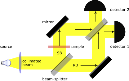
When light emitted from a source passes through a beam splitter, it splits into two beams with identical phases but different wavelengths. These beams then undergo mirror reflection and interference at the end, forming interference fringes. If there are different optical path differences in the two paths, the interference fringes will shift. Now, let's simplify the setup into a single optical fiber. The structure from left to right is as follows:

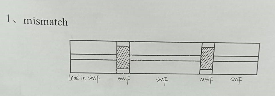
In the structure above, from left to right: single-mode fiber (SMF), multi-mode fiber (MMF), single-mode fiber, multi-mode fiber, single-mode fiber, and finally a connector. When light from the source enters the SMF, it propagates in the core, becoming single-mode light. It then enters the MMF and propagates in the cladding, splitting into two beams. These beams re-enter the SMF's cladding, propagate, enter the cladding of the second MMF, and finally overlap in the last segment of SMF, creating interference patterns.

It's important to note that during the transition from the core of the SMF to the cladding of the MMF, some light enters the core of the MMF; similarly, when transitioning from the cladding of the MMF to the cladding of the SMF, some light refracts into the core of the SMF. Direct propagation occurs from the core of the first SMF to the core of the last SMF. However, these do not affect the light propagating in the cladding that produces interference.

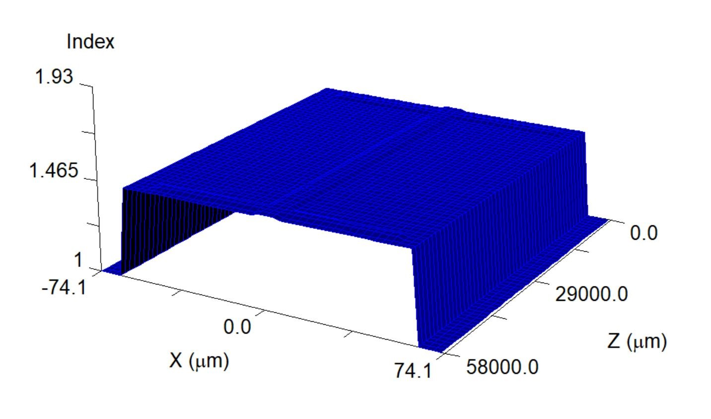
The outer diameter of the fiber is about 125 micrometers, and its length is a few centimeters. Therefore, the actual structure might resemble the following image:

Experiment design

If the lower half of the cladding of the middle SMF is placed in a temperature-adjustable liquid, the refractive index will change with temperature. This change in refractive index will cause different optical path differences between the two beams, resulting in the interference fringes at the end of the fiber moving. By measuring the distance of this movement, the change in temperature can be determined.

2. Computer Simulation

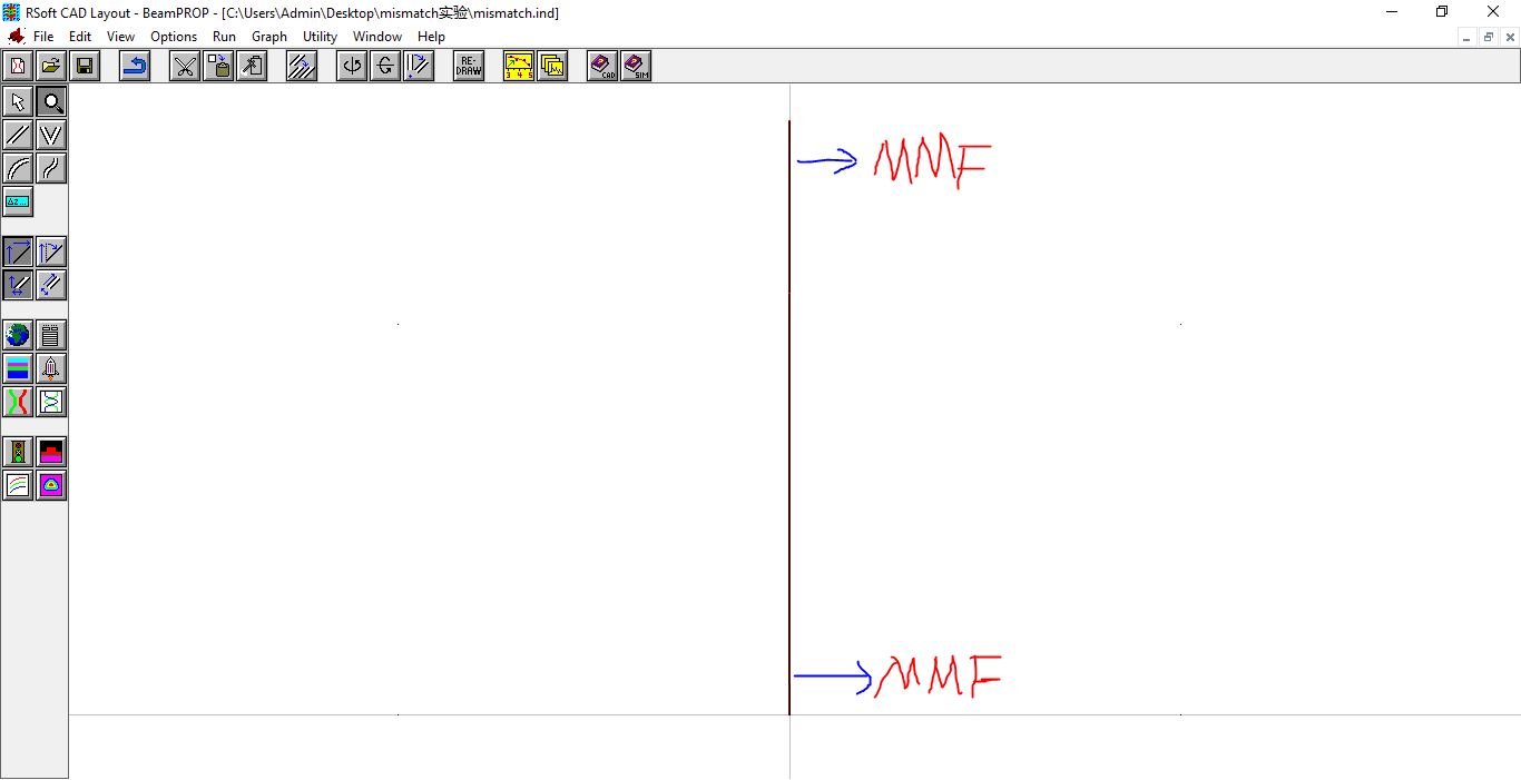
2.1 Use the finite element analysis tool Rsoft.

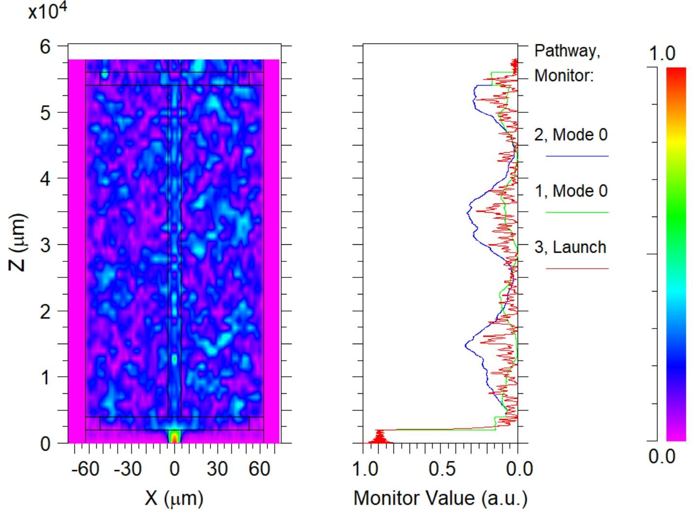
Download Rsoft, open /bin/bcadw32.exe, and run the mismatch.ind experiment file: [File]->[open]. Then click

->

to obtain the power distribution of the single-mode light:

2.2 Scan the distribution

Click

->

Assuming no refractive index difference between upper and lower claddings, and scan in the 1525-1565nm range to obtain the following:

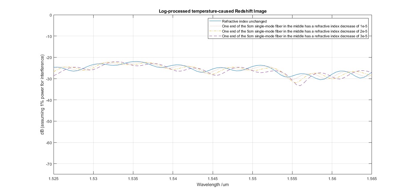
Next, vary the refractive index of the lower cladding by different values (based on quartz data, assume a refractive index change of 1e-5 per Celsius degree). Repeat the plotting as shown above and compile the data into /mismatch/MISMATCH data.txt. Use MATLAB for plotting:

Here's Matlab code above:

clear;
clc;
clf;
% Define wavelength range
x=1.525:0.0005:1.565;
% Original data arrays
y0=[3.4054255400 3.4406751496 3.2074056699 2.8028451365 2.4089229078 2.2276990773 2.3580537917 2.7616419517 3.3478593854 4.0124058938 4.5948707792 4.9171847603 4.9127349945 4.6679000439 4.3517753579 4.1599257418 4.2622131790 4.6955313978 5.3160983467 5.9066400101 6.2976141622 6.3792632616 6.0975092276 5.4999550032 4.7396749313 4.0080327520 3.4835261119 3.2982360827 3.4688532803 3.8585852989 4.2488135203 4.4490031712 4.3514012289 3.9506912929 3.3492196234 2.7146861188 2.2120906074 1.9668725862 2.0398128811 2.3836949550 2.8379247630 3.2018413605 3.3283799653 3.1797889303 2.8431380796 2.4934819945 2.3026624820 2.3626445991 2.6760391392 3.1724290296 3.7132803920 4.1233181170 4.2579284051 4.0515419999 3.5292538305 2.8100056711 2.0832214286 1.5280950885 1.2319383423 1.1840111325 1.3179899206 1.5304918666 1.6893123884 1.6873061283 1.5126440468 1.2501308882 1.0117348971 0.88566951562 0.93791745804 1.1995535128 1.6127881592 2.0221645165 2.2620175280 2.2511195528 2.0074992201 1.6238683328 1.2529101160 1.0603809340 1.1393879811 1.4766843821 1.9941608927];
y1=[2.9795846146 3.4165813368 3.5956409037 3.4615902919 3.0944361649 2.6811570000 2.3986753086 2.3588620673 2.6414103256 3.2635337868 4.0903829183 4.8683880643 5.3789822304 5.5263676064 5.3331948138 4.9432053890 4.5859837683 4.4450883242 4.5654614266 4.8999693377 5.3652624002 5.8194434815 6.0751901141 5.9957192133 5.5581641948 4.8463633855 4.0399276419 3.3767236847 3.0411006346 3.0688078475 3.3618714014 3.7545922119 4.0599295772 4.1226162669 3.8799098081 3.3754004664 2.7349604809 2.1445341558 1.7992413438 1.8076262005 2.1315455661 2.6178499295 3.0746243372 3.3436028700 3.3605252800 3.1710956720 2.8845205336 2.6209749884 2.4935661339 2.5828760274 2.8869112348 3.3066372910 3.6885213524 3.8764019545 3.7573692019 3.3163011764 2.6580873023 1.9527951396 1.3554847055 0.97531271877 0.87200981392 1.0264450076 1.3206089866 1.5910093703 1.7209822188 1.6783364917 1.4886896997 1.2196514322 0.99127653862 0.93975271306 1.1222696601 1.4690382566 1.8417712033 2.1148218813 2.2029228461 2.0766447985 1.7937082486 1.4835016672 1.2742499734 1.2514991254 1.4653894648];
y2=[2.0991150442 2.6655172720 3.1976215346 3.5218532602 3.5566372859 3.3414710636 2.9751573591 2.5963268959 2.4106812264 2.6123429171 3.2292500170 4.0995748233 4.9885446419 5.6752819168 5.9945991164 5.9111380684 5.5441134088 5.0704357361 4.6405051859 4.3926098688 4.4382715673 4.7682945599 5.2255707771 5.5941135893 5.6876197932 5.4013286069 4.7711024346 3.9819030545 3.2677297119 2.7997781253 2.6548014143 2.8157208309 3.1651286447 3.5195002565 3.7028406135 3.6005832904 3.1949854336 2.5958547694 2.0118753864 1.6453362393 1.5996217299 1.8610947730 2.3234551866 2.8293860492 3.2313342052 3.4356786747 3.4057705247 3.1650200712 2.8141521572 2.5061918628 2.3689945473 2.4471812812 2.6952698904 2.9919010001 3.1769841434 3.1264628260 2.8123503118 2.2934953419 1.6761449667 1.0997848131 0.71693412451 0.62517761628 0.80549823889 1.1423724572 1.4975299118 1.7530412711 1.8184842679 1.6637669872 1.3669175029 1.0884544419 0.96562456540 1.0401203805 1.2784747028 1.6104363243 1.9334126369 2.1369250884 2.1634395707 2.0295489145 1.7937628074 1.5457130940 1.4125541931];
y3=[1.3657344229 1.6580346704 2.1465199878 2.6956746434 3.1584278799 3.4253864117 3.4184110879 3.1396033964 2.7521128799 2.5201623807 2.6326383133 3.1221512679 3.9069240197 4.8173907615 5.6206309698 6.1203416602 6.2346484129 5.9684970678 5.3962003071 4.7060575569 4.1622116932 3.9532744484 4.0991396621 4.4793316857 4.8869760109 5.0928817960 4.9547268192 4.4862070325 3.8135343985 3.1026286590 2.5277415949 2.2299656366 2.2516807894 2.5173300314 2.8705174767 3.1228124784 3.1215096534 2.8317837891 2.3556179895 1.8617670416 1.5069281486 1.3980438513 1.5698623726 1.9749212230 2.5048923769 3.0193212247 3.3670181893 3.4345990659 3.2122366145 2.8030482058 2.3621143572 2.0311681559 1.8976437989 1.9617622026 2.1336275513 2.2855380586 2.3127136601 2.1526982803 1.7936593329 1.3026571165 0.82577089072 0.51795535930 0.46110037556 0.64732667792 1.0090522814 1.4324582551 1.7661436489 1.8820639488 1.7594730330 1.4914592229 1.2049028060 0.99907102031 0.94782527159 1.0944219359 1.4120633033 1.8028898533 2.1525698629 2.3664092315 2.3774391286 2.1861344791 1.8983895236];
y4=[1.1292898078 1.0530123926 1.1614868730 1.4777083316 1.9613177022 2.5139406208 2.9661806193 3.1542211712 3.0588811707 2.8207179961 2.6199121686 2.6011904606 2.8712992568 3.4557646861 4.2532342370 5.0852783143 5.7628455377 6.0966736451 5.9535047355 5.3761103375 4.5944629021 3.8857200372 3.4502066731 3.3725088080 3.5991741777 3.9514772744 4.2218924377 4.2686612226 4.0305056452 3.5254234776 2.8704317130 2.2527143038 1.8422942247 1.7257586616 1.8830349374 2.1876580982 2.4580407970 2.5542941265 2.4344513440 2.1372424049 1.7530033782 1.4081564837 1.2308404935 1.3048419122 1.6427017392 2.1701590759 2.7269961692 3.1240267656 3.2355803766 3.0460660174 2.6308047283 2.1207796821 1.6640762783 1.3698799979 1.2683837082 1.3210911041 1.4489564781 1.5454865779 1.5064423861 1.2921382438 0.96156948516 0.63192783901 0.41272582964 0.37889080761 0.56510794779 0.93757436987 1.3752731592 1.7228670263 1.8818471679 1.8406266292 1.6354250350 1.3305361383 1.0368719878 0.89022109895 0.97737780924 1.2965325300 1.7749002577 2.2837818083 2.6584838658 2.7767568055 2.6382968827];
y5=[0.90417651358 0.84872022000 0.82112537699 0.89390866429 1.1502888257 1.6024523493 2.1548855771 2.6899656970 3.0789277362 3.1958224168 3.0607587278 2.8233795276 2.6304398537 2.6432653380 2.9791792817 3.5662672207 4.2067282565 4.6999913387 4.8839555951 4.7019006928 4.2152869622 3.5467497865 2.8647919106 2.3436775439 2.0905607531 2.1250730492 2.3694276119 2.6701162727 2.8834705921 2.8992951145 2.6481883960 2.1952358694 1.7227512282 1.3890407972 1.2977341282 1.4806541890 1.8265016326 2.1555401577 2.3311289865 2.2568923643 1.9278592825 1.4830325898 1.1019356147 0.91208089792 0.97788619638 1.2563121720 1.6022081485 1.8767211716 2.0076301526 1.9743510075 1.8047971693 1.5583577196 1.2788149614 0.99778046955 0.77810163225 0.69155444707 0.75175295657 0.90253075984 1.0453498211 1.0784311285 0.96007164964 0.72650559781 0.46127602432 0.28598801327 0.30785521226 0.53030588398 0.86500507906 1.2025185796 1.4398554270 1.5047409203 1.3874532191 1.1397663137 0.84540443253 0.58857386000 0.45216280215 0.52720297016 0.86510117977 1.4153415381 2.0581085342 2.6639913549 3.0851902997];
y6=[0.49349269594 0.61095545420 0.67268870387 0.66728251988 0.66316598483 0.76570268357 1.0444405281 1.5336180414 2.1682917960 2.7558457361 3.1318177575 3.2203664311 3.0118361283 2.6537403218 2.3907337453 2.3667610093 2.5955929014 2.9938305670 3.4018989698 3.6720701759 3.7137832009 3.4939685680 3.0651920606 2.5436282232 2.0574000507 1.7287135159 1.6305699955 1.7573859082 2.0553606637 2.4010572812 2.6018409898 2.5382631475 2.2271705077 1.7562101441 1.2922797207 1.0373160467 1.0799756195 1.3824569284 1.8218151073 2.1847559548 2.2866167199 2.0988071909 1.7074674260 1.2601395789 0.93167193439 0.81836326121 0.89387797233 1.0834761674 1.3115587371 1.5064805564 1.6242276755 1.6459369186 1.5446666153 1.3083682023 0.99635570442 0.71802821676 0.56259303487 0.56666657324 0.69785837738 0.86418591416 0.97055235834 0.94864101524 0.78132616931 0.54887086249 0.38141622591 0.35914611501 0.49941880052 0.77245159622 1.0957564738 1.3647317060 1.5031430759 1.4873415368 1.3379429679 1.0993908991 0.85003597874 0.71547824466 0.80935379235 1.1640979719 1.7506887090 2.4901979643 3.2042795284];
y7=[0.13695246934 0.36688114448 0.64768702741 0.86870643008 0.96196573590 0.94007678178 0.87782682350 0.93340578168 1.2441476452 1.7909853197 2.4541519391 3.0428195304 3.3262919937 3.2277009237 2.8653756128 2.4139143282 2.0475075112 1.8881694396 1.9528939587 2.1894014550 2.5028349853 2.7763489250 2.9255531582 2.9076493370 2.7159165654 2.4063091328 2.0759753592 1.8318197296 1.7974879245 2.0208505968 2.3821488108 2.7009353225 2.8232533392 2.6250981300 2.1286194260 1.5314720304 1.0577443289 0.88657268864 1.0911490799 1.5438860055 2.0080182853 2.2935696858 2.2928943680 2.0175263381 1.6082024852 1.2205684233 0.94428769770 0.82809689274 0.88639935386 1.0850336195 1.3661684750 1.6535961935 1.8305236884 1.7928567140 1.5395513384 1.1651546782 0.80081668188 0.57597066368 0.56099614536 0.73687001288 1.0148233615 1.2481507335 1.3043649309 1.1699026088 0.92606615756 0.67614104409 0.53294285026 0.58046702359 0.81689346489 1.1626119143 1.5100648500 1.7688407731 1.8802784787 1.8178079321 1.6207146410 1.4072209041 1.2997282693 1.3747947400 1.6980276272 2.2883298819 3.0210262860];
% Convert to logarithmic scale in dB (assuming 1% of power is used for interference)
Y0=10*log10(0.001*y0); 
Y1=10*log10(0.001*y1);
Y2=10*log10(0.001*y2);
Y3=10*log10(0.001*y3);
Y4=10*log10(0.001*y4);
Y5=10*log10(0.001*y5);
Y6=10*log10(0.001*y6);
Y7=10*log10(0.001*y7);

% Plot each data set with logarithmic scale
plot(x,Y0);
xlabel('Wavelength /um');
ylabel('dB (assuming 1% power for interference)');
title('Log-processed temperature-caused Redshift Image');
grid on;
axis([1.525,1.565,-75,0]);
pause(0.2);

plot(x,Y1);
xlabel('Wavelength /um');
ylabel('dB (assuming 1% power for interference)');
title('Log-processed temperature-caused Redshift Image');
grid on;
axis([1.525,1.565,-75,0]);
pause(0.2);

plot(x,Y2);
xlabel('Wavelength /um');
ylabel('dB (assuming 1% power for interference)');
title('Log-processed temperature-caused Redshift Image');
grid on;
axis([1.525,1.565,-75,0]);
pause(0.2);

plot(x,Y3);
xlabel('Wavelength /um');
ylabel('dB (assuming 1% power for interference)');
title('Log-processed temperature-caused Redshift Image');
grid on;
axis([1.525,1.565,-75,0]);
pause(0.2);

plot(x,Y4);
xlabel('Wavelength /um');
ylabel('dB (assuming 1% power for interference)');
title('Log-processed temperature-caused Redshift Image');
grid on;
axis([1.525,1.565,-75,0]);
pause(0.2);

plot(x,Y5);
xlabel('Wavelength /um');
ylabel('dB (assuming 1% power for interference)');
title('Log-processed temperature-caused Redshift Image');
grid on;
axis([1.525,1.565,-75,0]);
pause(0.2);

plot(x,Y6);
xlabel('Wavelength /um');
ylabel('dB (assuming 1% power for interference)');
title('Log-processed temperature-caused Redshift Image');
grid on;
axis([1.525,1.565,-75,0]);
pause(0.5);

plot(x,Y7);
xlabel('Wavelength /um');
ylabel('dB (assuming 1% power for interference)');
title('Log-processed temperature-caused Redshift Image');
grid on;
axis([1.525,1.565,-75,0]);
pause(0.2);
  
plot(x,Y0,'-',x,Y1,':',x,Y2,'-.',x,Y3,'--');
xlabel('Wavelength /um');
ylabel('dB (assuming 1% power for interference)');
title('Log-processed temperature-caused Redshift Image');
grid on;
axis([1.525,1.565,-75,0]);
legend('Refractive index unchanged', 'One end of the 5cm single-mode fiber in the middle has a refractive index decrease of 1e-5', 'One end of the 5cm single-mode fiber in the middle has a refractive index decrease of 2e-5', 'One end of the 5cm single-mode fiber in the middle has a refractive index decrease of 3e-5');

3. Measure by experiment

Based on the optical power analyzer for pigtails, the actual image is as follows: